Medical Imaging | InceptionV3

---

KEYWORDS
TensorFlow, Deep Learning, CNN, Inception Architecture, Medical Imaging, Image Classification, Supervised Learning

---

Introduction

• Pneumonia is a leading cause of death worldwide, responsible for millions of deaths each year. Chest X-rays are the standard diagnostic tool, but interpreting them is time-consuming and prone to human error.
  • In recent years, deep learning, particularly convolutional neural networks (CNNs), has emerged as a powerful alternative for medical image analysis.

• Among various models, fine-tuned Inception-v3 networks have achieved impressive results, with studies reporting up to 99% accuracy in pneumonia classification tasks (reference).

• In this post, I describe how I built and trained a CNN inspired by InceptionV3, using Keras and TensorFlow, to classify chest X-ray images as either pneumonia or normal.
  • My goal is not only to achieve high accuracy but also to explore the unique challenges involved in applying deep learning to real-world medical data.

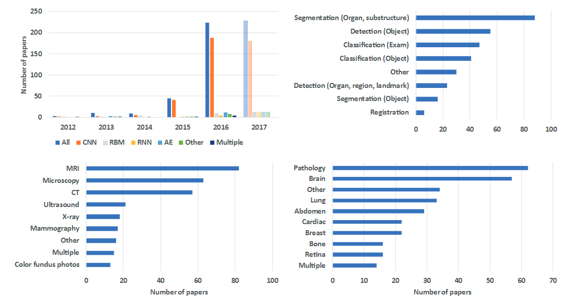Number of Papers in medical AI field [^8]

Background on InceptionV3

• Inception-v3, introduced by Szegedy et al. (2015), is a deep CNN architecture designed for efficiency and high accuracy (reference). Key innovations include:

  • Factorized/Asymmetric Convolutions: Large filters are broken into smaller ones (e.g., 5×5 into two 3×3, or 3×3 into 1×3 + 3×1) to reduce parameters (reference).
  • Auxiliary Classifier: A side branch added mid-network helps improve gradient flow and regularization during training (reference).
  • Other Techniques: Label smoothing, batch normalization, and efficient grid-size reductions further boost performance (reference).

• These improvements make Inception-v3 both powerful and computationally efficient compared to earlier models.

Dataset and Preprocessing

• I used the public “Chest X-Ray Images (Pneumonia)” dataset (Kaggle), containing X-rays labeled NORMAL or PNEUMONIA. Data were organized into train, val, and test folders by class. The training set was imbalanced (3875 pneumonia vs. 1341 normal cases) (reference).

• Images were loaded and preprocessed using Keras’s ImageDataGenerator: resized to 150×150, normalized (rescale=1./255), and batched (batch size 64).

  • Notably, the validation split was very small (only 16 images), while a separate test set of 624 images was reserved for final evaluation.

  • This pipeline produced ready-to-train batches for the model.

train_datagen = ImageDataGenerator(rescale=1./255)
val_datagen = ImageDataGenerator(rescale=1./255)

train_generator = train_datagen.flow_from_directory(
    train_path,
    target_size=(150, 150),
    batch_size=64,
    class_mode='binary'
)

val_generator = val_datagen.flow_from_directory(
    val_path,
    target_size=(150, 150),
    batch_size=64,
    class_mode='binary'
)

Model Architecture and Fine-Tuning

• My model is a custom Inception-v3-like network built with the Keras functional API. We defined an inception_module that performs parallel convolutions (1×1, 3×3, 5×5) and pooling, as in the original design (reference here). Concretely, each module has four branches:
  • 1×1 convolution,
  • a 1×1 followed by factorized 3×3 convolution (implemented as 3×1 then 1×3) (reference here),
  • a 1×1 followed by factorized 5×5 convolution (5×1 + 1×5) (reference here), and
  • 3×3 max pooling followed by a 1×1 conv (pool projection) (reference here).

def inception_module(x, filters):
    f1, f2_in, f2_out, f3_in, f3_out, f4_out = filters

    conv1x1 = Conv2D(f1, (1,1), padding='same', activation='relu')(x)

    conv3x3 = Conv2D(f2_in, (1,1), padding='same', activation='relu')(x)
    conv3x3 = Conv2D(f2_out, (3,1), padding='same', activation='relu')(conv3x3)
    conv3x3 = Conv2D(f2_out, (1,3), padding='same', activation='relu')(conv3x3)

    conv5x5 = Conv2D(f3_in, (1,1), padding='same', activation='relu')(x)
    conv5x5 = Conv2D(f3_out, (5,1), padding='same', activation='relu')(conv5x5)
    conv5x5 = Conv2D(f3_out, (1,5), padding='same', activation='relu')(conv5x5)

    pool = MaxPooling2D((3,3), strides=1, padding='same')(x)
    pool = Conv2D(f4_out, (1,1), padding='same', activation='relu')(pool)

    output = Concatenate()([conv1x1, conv3x3, conv5x5, pool])

    return output

• I stacked two Inception modules sequentially, with filter sizes [64,48,64,8,16,32] and [128,64,96,16,32,64] (reference).

• An auxiliary classifier was attached afterward: it applies 5×5 average pooling (stride 3), a 1×1 convolution, flattens the feature maps, and passes through a dense layer (128 units, ReLU) with 50% dropout.

• The final auxiliary output is a single sigmoid neuron (aux_output) used for binary classification (reference).

def auxiliary_classifier(x, num_classes):
    x = AveragePooling2D((5,5), strides=3)(x)
    x = Conv2D(64, (1,1), activation='relu')(x)
    x = Flatten()(x)
    x = Dense(128, activation='relu')(x)
    x = Dropout(0.5)(x)
    x = Dense(num_classes, activation='sigmoid', name="aux_output")(x)
    return x

def inception_v3(input_shape, num_classes=1):
    inputs = Input(shape=input_shape)

    x = Conv2D(32, (3,3), strides=2, padding='valid', activation='relu')(inputs)
    x = Conv2D(32, (3,3), padding='valid', activation='relu')(x)
    x = Conv2D(64, (3,3), padding='same', activation='relu')(x)
    x = MaxPooling2D((3,3), strides=2, padding='valid')(x)

    x = inception_module(x, [64, 48, 64, 8, 16, 32])
    x = inception_module(x, [128, 64, 96, 16, 32, 64])

    aux_output = auxiliary_classifier(x, num_classes)

    x = GlobalAveragePooling2D()(x)
    x = Dense(128, activation='relu')(x)
    x = Dropout(0.5)(x)

    model = Model(inputs, aux_output)
    return model

• After defining the layers, I compiled the model with the Adam optimizer and binary cross-entropy loss (matching our single sigmoid output), I also optimized the model using binary cross-entropy loss:

\(\mathcal{L} = -\frac{1}{N} \sum_{i=1}^{N} \left( y_i \log(p_i) + (1 - y_i) \log(1 - p_i) \right)\)

where \((y_i)\) is the true label and \((p_i)\) is the predicted probability.

• No other data augmentation was applied in this run. In summary, the network structure mirrors InceptionV3’s design: parallel multi-scale convolutional paths and an auxiliary classifier for regularization, adapted for two-class pneumonia detection (reference here) (reference here).

model.compile(optimizer='adam',
                 loss={'aux_output': 'binary_crossentropy'},
                 metrics=['accuracy'])

Training and Evaluation

• I trained the model on a GPU for 5 epochs, using the full training set and validating on a small validation split (reference).

  • Training accuracy quickly rose to ~93.8% by epoch 4, but validation accuracy peaked at ~75.0% before dropping to ~62.5% in epoch 5, suggesting overfitting (reference).

• On the separate 624-image test set, the model achieved 76.44% accuracy (reference). Sensitivity to pneumonia was high (recall 0.99), but normal class recall was low (0.38) (reference). Precision was 0.98 for normal cases and 0.73 for pneumonia.

  • Overall, the model favored predicting pneumonia, resulting in a weighted F1 score of about 0.73.

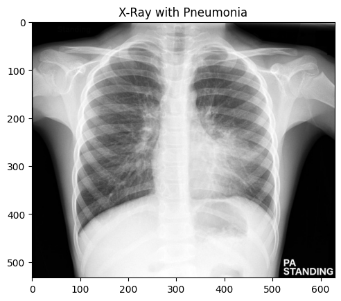#https://radiopaedia.org/cases/childhood-pneumonia-1 [^8]

prediction = model.predict(img_array)

if prediction[0][0] > 0.5:
    print("Pneumonia")
else:
    print("Normal")

Pneumonia

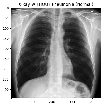#https://radiopaedia.org/cases/normal-chest-x-ray [^8]

prediction = model.predict(img_array)

if prediction[0][0] > 0.5:
    print("Pneumonia")
else:
    print("Normal")

Normal

Challenges and Learnings

• Class imbalance: The data had far more pneumonia cases than normals (3875 vs 1341 in training) (reference here). This likely biased the model towards predicting pneumonia.

  • Indeed, our confusion report showed very high pneumonia recall (0.99) but poor normal recall (0.38) (reference here). Techniques like class weighting or targeted augmentation of the minority class might improve this.

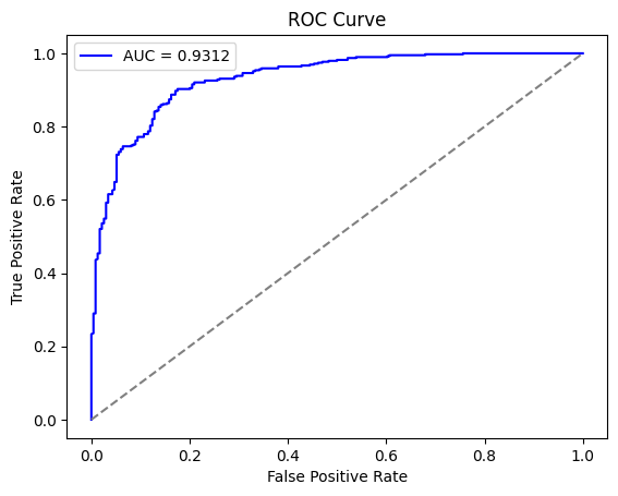
from sklearn.metrics import roc_curve, auc

probabilities = model.predict(test_generator)

fpr, tpr, _ = roc_curve(true_labels, probabilities)
roc_auc = auc(fpr, tpr)

plt.figure()
plt.plot(fpr, tpr, color='blue', label=f'AUC = {roc_auc:.4f}')
plt.plot([0, 1], [0, 1], color='gray', linestyle='--')
plt.xlabel("False Positive Rate")
plt.ylabel("True Positive Rate")
plt.title("ROC Curve")
plt.legend()
plt.show()

• Overfitting: Training accuracy was much higher than validation, with validation peaking at ~75% by epoch 4 before declining (reference).

• Even with only 5 epochs, the model showed signs of memorization.

• More regularization (e.g., dropout, early stopping) or additional data would help close the train/validation gap.

• Limited Validation Data: The validation set was extremely small (16 images) (reference), making the metrics noisy and unreliable.

• A larger validation split or cross-validation would provide better feedback. More data or data augmentation could also improve generalization.

• Training Stability: Warnings appeared about the Dataset running out of data, likely due to the tiny validation generator (reference).
  • Ensuring correct steps_per_epoch and validation_steps, or using dataset repeats, would improve stability.
• These challenges highlight that while the Inception-like model is expressive, successfully applying it to chest X-rays requires careful handling of data imbalance, augmentation, and possibly transfer learning.

Conclusion

• I demonstrated an InceptionV3-inspired CNN for pneumonia detection on chest X-rays, achieving about 76.4% test accuracy. The model showed high sensitivity for pneumonia but low specificity for normal cases.

• While this provides a reasonable baseline, it falls short of the >96% accuracy reported in studies using pretrained models, stronger augmentation, or ensembling (reference).

  • Future improvements could include transfer learning, enhanced data augmentation, hyperparameter tuning, and model ensembling.
  • Deep CNNs like InceptionV3 are powerful for automated screening, but clinical-grade performance demands more data and careful optimization.

References